
4. Results of multi-level analysis of ECEC reforms and educational inequality
In this chapter, we will focus on the association between ECEC reforms and development in measures of educational inequality, using TIMSS and PIRLS data. We will, based on a selection of certain reforms that can be seen as comparable in goals and target groups (see chapter 3 for an overview of these), investigate the difference in development in inequality between countries which implemented such reforms during a chosen period, and countries that did not. We will first show descriptive findings showing the development in inequality between certain groups for before and after the reforms and then show multi-level models where we examine the association between reforms and the development of inequality. Despite the analysis being descriptive, it will still serve as an overview of how we can understand the implementation of reforms in different countries, and how they did, or did not, change the patterns of inequality in the respective countries.
4.1. Reforms
We have chosen to focus on reforms which target preschool children (ISCED level 0), and are aimed at granting/expanding access to ECEC, targeting inequalities explicitly. This means that we leave out reforms collected in WP2 which focus on special needs, curricula adjustments, teachers or education levels (and thus, children) above ISCED 0. Maintaining a strict focus on inequality serves to facilitate comparison between countries, as well as keeping the analysis within the focus of the STRIDE project. As inequality can be present in many dimensions, we include measures of parental education, gender, urban/rural and immigrant background in our analyses, following the focus in chapter 3. The reforms we have included in this analysis have been implemented at different time-points, and to facilitate descriptions of the different reforms and their relationships to inequality measures, we chose reforms that were introduced between 2006 and 2018, so that we have survey data on test-scores available from five years before and after the reforms, as well. In this way, we acknowledge that the rolling out, implementation and impact of a reform takes time. For our analysis, we matched the pre- and post-reform period, as well as the year of the reform to both TIMSS and PIRLS waves. For countries that did not have any reforms in this period, we included the data from the mean years used in the countries with a reform. The countries with their corresponding reform years and waves of data are listed below, in Table 4.1.[1]
Table 4.1: Countries, year of ECEC reform, years before and after, waves of PIRLS and TIMSS data used
| Country | Year (t) | t-5 | t+5 | PIRLS t1 | PIRLS t2 | PIRLS t3 | TIMSS t1 | TIMSS t2 | TIMSS t3 |
|---|---|---|---|---|---|---|---|---|---|
| Belgium – Flemish | 2009 | 2004 | 2014 | — | — | — | 2003 | 2011 | 2015 |
| Bulgaria | 2009 | 2004 | 2014 | 2006 | 2011 | 2016 | — | — | — |
| Denmark | 2007 | 2002 | 2012 | — | — | — | — | — | — |
| Germany | 2008 | 2003 | 2013 | 2001 | 2006 | 2016 | — | — | — |
| Ireland | 2010 | 2005 | 2015 | — | — | — | — | — | — |
| Greece | 2018 | 2013 | 2023 | — | — | — | — | — | — |
| France | 2013 | 2008 | 2018 | 2006 | 2011 | 2021 | — | — | — |
| Croatia | 2014 | 2009 | 2019 | — | — | — | 2011 | 2015 | 2019 |
| Italy | 2017 | 2012 | 2022 | 2011 | 2016 | 2021 | 2011 | 2015 | 2023 |
| Latvia | 2013 | 2008 | 2018 | — | — | — | 2003 | 2007 | 2019 |
| Hungary | 2015 | 2010 | 2020 | 2011 | 2016 | 2021 | 2011 | 2015 | 2023 |
| Malta | 2017 | 2012 | 2022 | 2011 | 2016 | 2021 | — | — | — |
| Austria | 2010 | 2005 | 2015 | 2006 | 2011 | 2016 | 2007 | 2011 | 2019 |
| Poland | 2011 | 2006 | 2016 | 2006 | 2011 | 2016 | — | — | — |
| Portugal | 2018 | 2013 | 2023 | 2011 | 2016 | 2021 | 2015 | 2019 | 2023 |
| Romania | 2016 | 2011 | 2021 | — | — | — | — | — | — |
| Slovenia | 2008 | 2003 | 2013 | 2001 | 2006 | 2016 | 2003 | 2007 | 2015 |
| Slovakia | 2015 | 2010 | 2020 | 2011 | 2016 | 2021 | 2011 | 2015 | 2023 |
| Finland | 2015 | 2010 | 2020 | 2011 | 2016 | 2021 | 2011 | 2015 | 2023 |
| Norway | 2009 | 2004 | 2014 | 2006 | 2011 | 2016 | 2003 | 2007 | 2015 |
| England | 2010 | 2005 | 2015 | 2006 | 2011 | 2016 | 2007 | 2011 | 2015 |
Table 4.2: Selected PIRLS and TIMSS waves for countries without ECEC reform in chosen period
| Country | PIRLS t1 | PIRLS t2 | PIRLS t3 | TIMSS t1 | TIMSS t2 | TIMSS t3 |
|---|---|---|---|---|---|---|
| Czech Republic | 2001 | 2011 | 2016 | 2007 | 2011 | 2019 |
| Spain | 2006 | 2011 | 2016 | 2011 | 2015 | 2019 |
| Cyprus | — | — | — | 2003 | 2015 | 2019 |
| Lithuania | 2006 | 2011 | 2016 | 2007 | 2011 | 2019 |
| Netherlands | 2006 | 2011 | 2016 | 2007 | 2011 | 2019 |
| Sweden | 2006 | 2011 | 2016 | 2007 | 2011 | 2019 |
The sample of this analysis is made up of 17 countries with a relevant reform during the chosen period, and 6 countries without (see countries listed in table 4.1 and 4.2). The time of the adoption of the reforms spans from 2007 to 2018. We included test scores (and other variables) five years before and five years after the reform, in reading and mathematics. Reform implementation is shaped by multiple factors, and countries may display varying levels and trajectories of inequality that are independent of reform timing. The absence of a reform within the observed period may indicate that reforms were enacted shortly before our measurement window or that broader political preferences make reform adoption more or less likely. Changes in inequality before and after reforms do not necessarily reflect the impact of the reforms themselves. However, by presenting both descriptive trends and models that incorporate reform timing, we can identify whether any descriptive shifts in inequality follow these reforms. The insights may be relevant from a policy perspective, even if they cannot be interpreted causally.
4.2. Variables and descriptive trends
The main variables we are using are measures of reading and mathematics, based on PIRLS and TIMSS. We also use variables for gender, socioeconomic status (SES), immigration status, and school location. As addressed in previous sections, in these datasets, the gender variable has two values (i.e. boys and girls). SES is constructed based on information about parents, and has two values, one for no parents or guardians with a higher education degree and one for one or more parents or guardians with a higher education degree. Immigrant status is based on information about where the respondent is born and has the value 1 for children born in another country than the test and 0 for children born in the same country as the test. School location measures the centrality of the school, and has the value 0 for rural, meaning up to 15,000 people live in area, and 1 for not rural, meaning more than 15,000 people live in the area. Based on these variables we used an indicator of inequality constructed for the STRIDE-project earlier, which measures the ratio of the test score means by social group breakdown categories (for more details, see Steinmann et al., 2025). The ratio reflects how much higher one group scores compared to another, on average.
All indicators were constructed accounting for the complex sampling design of the surveys by including complex weights and plausible values (the latter was done according to Rubin’s (1987) rules). This enabled the computation of standard errors and confidence intervals.
First, we show some figures depicting the mean trends in inequality in all countries across the selected variables. The figures show the ratio of the test score means by social groups at three time-points: (a) the survey wave closest to five years before reform, (b) the year of reform and (c) five years after reform. As mentioned above, for countries which did not have a reform in the given time period, we used the mean year of the countries with a reform. This choice comes with its limitations, as we cannot know how using a different set of years for comparison impacts our analysis. However, we still believe the mean year is the best choice for comparison between countries, given that we use years that are not very far from each other in time. Still, this limitation should be kept in mind when analysing the results.
Source: own calculations based on TIMSS G4.
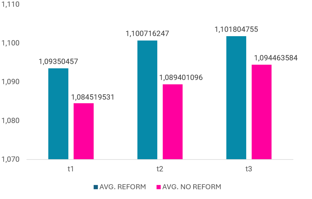
Figure 4.1 shows inequality by SES before, at the time of and after reforms for countries with and without reforms. For all countries, there has been an increase in this sort of inequality, seen in the rising number across bars. This is in line with the general increasing inequality in the period (Clarke et al., 2022) and a corresponding increase in educational inequality in the same period (OECD, 2024). The ratio changes from 1,094 to 1,102 for the countries with a reform, and from 1,085 to 1,094 for the countries without a reform, translating to a between 8 and 10% difference between students with highly educated parents and students without highly educated parents in all groups. The increase thus seems to be somewhat larger in the countries without a reform, but the difference is small (the difference between t1 and t3 is 0.08 with reform and 0.09 without).
Source: own calculations based on TIMSS G4.
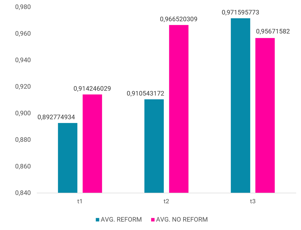
As for inequality according to immigrant background, Figure 4.2 shows that this has also increased in the period, but more so for the countries with a reform than the countries without a reform. The average change in ratio from t1 to t3 here is 0.79 in countries with a reform and 0.43 for the countries without. It has to be noted here, that given the descriptive nature of the analysis, the patterns observed may arise from multiple factors unrelated to the reforms themselves; for instance, demographic shifts such as changes in the proportion/composition of immigrant students within each country.
Source: own calculations based on TIMSS G4.
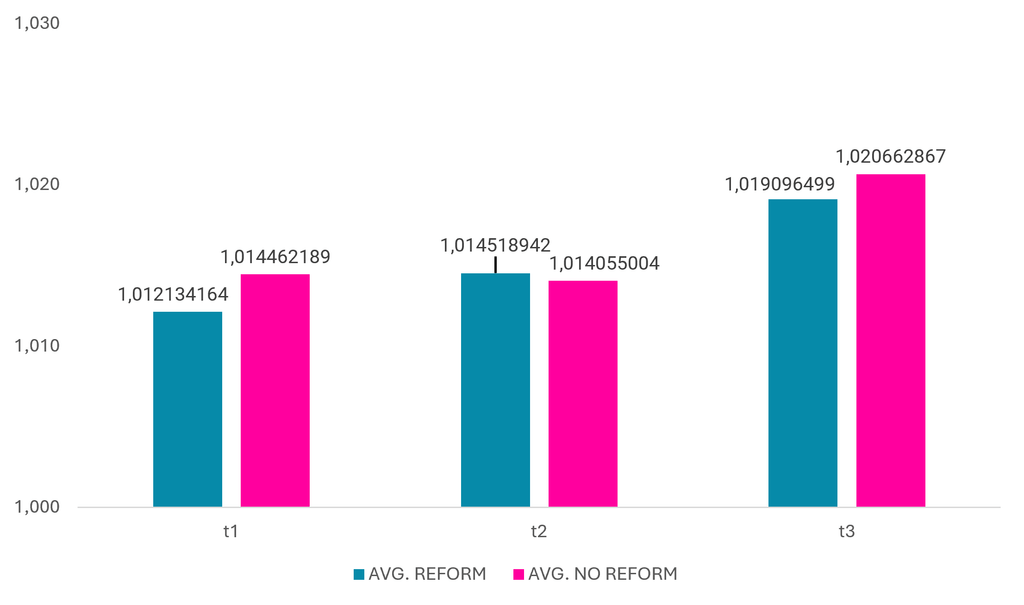
Finally, the figure on gender ratios (Figure 4.3) demonstrates that gender-related inequality remains very low in all countries and rises only marginally over time, with no distinction between those that enacted reforms and those that did not. This is consistent with the fact that the reforms in question did not explicitly address gender differences.
4.3. Results of multi-level analysis
The following section presents the findings from the multi-level analysis. In model 1, we interact reform status with parental education, modelling schools as level 2 units and countries as level 3 units. This structure enables us to examine whether reforms correspond to distinct patterns in the development of inequality. As the data is hierarchical in nature (students are nested in schools and; in turn, schools are nested in countries) we apply a multi-level model, as suggested in such instances (Gelman and Hill, 2007). We model test scores at t3 (five years after reform) as the dependent variable. Using a multi-level structure with schools as level 2 units and countries as level 3 units allows the intercepts to vary across both contexts. This approach estimates the individual and group-level components simultaneously, consistent with the “partial pooling” framework described by Gelman and Hill (2007). Although at least 25 units per level is commonly recommended, it is typical in cross-national research to have fewer units at the country level.
We include a dummy variable measuring if the country had a reform or not and interact it with parental education. We also control for gender, school location and immigrant background. We include relevant weights and first ran the model separately for the 5 plausible values, before we combined them into one model (using Rubin’s rules).
Table 4.3: Coefficients from 3-level regression model with students as level 1, schools as level 2 and countries as level 3
| Variable | Coefficient | Standard error | z-statistic | p-value | 95% confidence interval |
|---|---|---|---|---|---|
| Reform | -12.50* | 5.45 | -2.29 | 0.022 | [-23.18, -1.82] |
| Parental higher education | 25.47*** | 1.89 | 13.51 | 0.000 | [21.77, 29.16] |
| Reform × Parental higher education | 9.52*** | 2.37 | 4.01 | 0.000 | [4.87, 14.16] |
| Female | 10.23*** | 1.44 | 7.12 | 0.000 | [7.41, 13.05] |
| Immigrant | -25.97*** | 2.08 | -12.50 | 0.000 | [-30.05, -21.90] |
| Urban | 7.55* | 3.62 | 2.09 | 0.037 | [0.46, 14.65] |
| Constant | 535.83*** | 3.39 | 158.19 | 0.000 | [529.19, 542.47] |
| Random Parameters | |||||
| lnσ₁ (constant) | 2.68*** | 0.15 | 17.83 | 0.000 | [2.38, 2.97] |
| lnσ₂ (constant) | 3.22*** | 0.08 | 40.95 | 0.000 | [3.07, 3.37] |
| lnσₑ (constant) | 4.10*** | 0.02 | 205.09 | 0.000 | [4.06, 4.14] |
Table 4.3 shows that, similar to the descriptive figure 4.1, on average, the results are lower in the countries that had a reform than those that did not, that results are higher for those with parents with higher education, that girls do better than boys, that native children get better results than those with an immigrant background and that those that go to an urban school do better than those that go to a rural school. More importantly, the interaction between reform and parents’ education level is significant and positive, showing that inequality levels were higher in countries with a reform. As this model does not include any measures of student performance before and after the reforms, it is difficult to determine the underlying reasons for the observed patterns. It does, however, imply that those who have parents with higher education are not negatively affected by the reforms in the same way as those with parents without higher education.
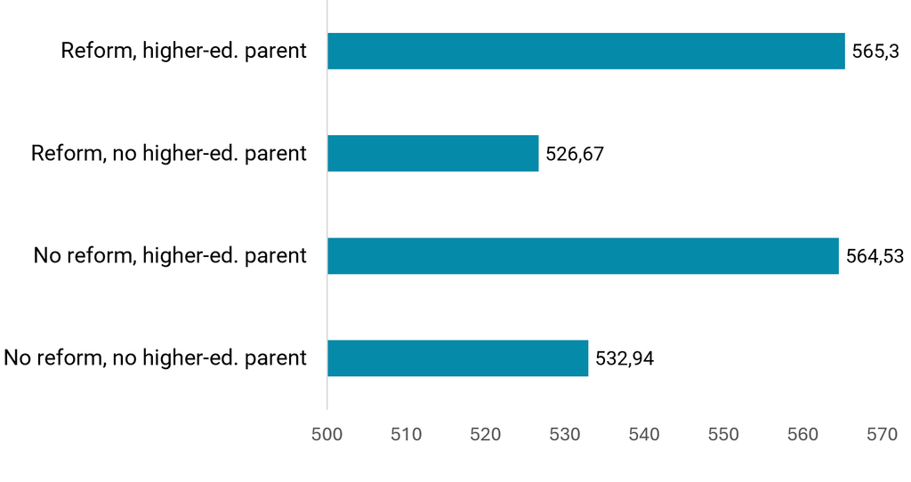
The predicted values based on Table 4.3, shown in Figure 4.4, confirm that test scores are lower for students in countries with reforms in the period, but also show that this difference only exists for students with parents with no higher education. A possible interpretation of these results is that the inequality level is the underlying concern for implementing a reform in the first place, as inequality is higher in the countries with reforms (the gap between the predicted test scores of the two groups is 39 in the case of countries with a reform, and only 32 for countries without a reform).
In the next model (model 2), we include the time-dimension to assess how an educational reform at the pre-school level might have had an impact on the individuals in the countries. We do this by including the three time points: before reform, at the time of reform and after reform, and interact the reform variable with parents’ education level. Here, at the waves corresponding to t1 and t2, the reform dummy is set to 0 for all countries, and at t3, it is set to 1 for countries which had a reform, and to 0 for countries which did not. In this model, the dependent variable is test score in the given wave, and we include country and year fixed effects and also control for gender, school location and immigrant background. Consequently, this construct shows the differences between countries which had and did not have a reform and how it has impacted inequality according to parents’ education level five years after the reform.
Table 4.4: Coefficients from linear regression model with country and year fixed effects, controlled for waves (Standard errors clustered on schools)
| Term | Level | Coef. | Std. Err. | t | P-Value | 95% CI (Lower) | 95% CI (Upper) |
|---|---|---|---|---|---|---|---|
| Reform_t3 | 1 | 12.792 | 1.928 | 6.630 | 0.000 | 8.992 | 16.593 |
| Parent HE | 1 | 35.529 | 0.583 | 60.960 | 0.000 | 34.383 | 36.675 |
| Reform_t3 × Parent_HE | 1 × 1 | 7.909 | 1.205 | 6.560 | 0.000 | 5.536 | 10.282 |
| Female | 1 | 10.796 | 0.388 | 27.850 | 0.000 | 10.036 | 11.556 |
| Immigrant | 1 | -29.025 | 0.553 | -52.490 | 0.000 | -30.116 | -27.933 |
| Urban | 1 | 5.777 | 0.786 | 7.350 | 0.000 | 4.235 | 7.318 |
| Constant | — | 517.836 | 2.341 | 221.230 | 0.000 | 513.218 | 522.453 |
Table 4.4 shows the output from the second model where we assess the differences in inequality between countries which had and did not have a reform at ISCED level 0. The output shows that when we add the time-dimension, having had a reform is positive and significant for the results. Moreover, the interaction-term between reform and parents’ education is also positive and significant, implying that the lifting effect of a reform is higher for students with parents with higher education. This means that even if the reform lifts all students on average, it does not reduce social inequality in results; it rather amplifies it.
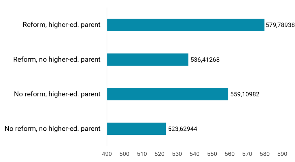
Figure 4.5 containing the predicted values for the interaction term confirms the findings in model 2, table 4.4. Having had a reform increases the results for all groups, but more so for those with parents with higher education than for those with parents without higher education. Thus, the reforms do not, in the time-perspective we apply here, decrease the inequality in results between students with and without higher-educated parents. However, we do not know whether or not a reduction of inequalities might occur at a later time point, as suggested by some studies.
Discussion of findings
A common finding in the literature on education and inequality is that increased schooling is more advantageous for children with lower SES (see e.g., Raudenbusch and Eschmann, 2015), and our findings can be interpreted to be differing from that. However, our models are not necessarily showing the impact of more years of education, as we merely measure how the implementation of reforms matter for the results of children five years after in the same country. Future research should examine how the specific reforms impact children who were affected by the reform, and how this differs by SES and other measures of inequality. We did, however, show that the reforms seem to be correlated with an improvement of results for everyone, even if somewhat more so for those with higher SES.
Notes
- In the case of some countries (Denmark, Ireland, Greece, Romania), even though they did have a reform in the period, it was not possible to match the time points to survey waves, due to lack of data. ↩